Answer:
To quickly view different worksheets on your dashboard, you will need to set up a parameter and calculation and then place the worksheets onto your dashboard and remove the title.
Here are the steps you will use.
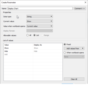
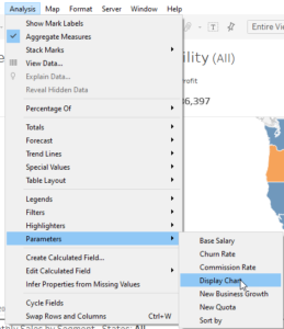
Step 1: Create a Parameter
– Create a Parameter: ‘Display Chart’
– Data type: String
– Allowable values: List
– Values:
– 1st Chart Name Here (type the name of your 1st sheet)
– 2nd Chart Name Here (type the name of your 2nd sheet)
– Click Ok
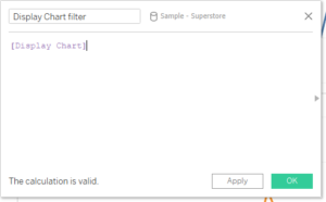
Step 2: Create a Calculation to run the Parameter
– Create a calculation: ‘Display Chart Name’ and add the parameter field
– [Display Chart]
– Click Ok
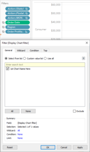
Step 3: Add the parameter calculation to the ‘Filter card’ of the 1st worksheet
– Select ‘1st Chart Name’ and ‘Ok’
Note: the view is displayed
Step 4: Add the parameter calculation to the ‘Filter’ on the second worksheet
– Select Custom Calculation and type ‘2nd Chart Name Here’, hit the (+) sign to add and ‘Ok’
Note: the view will disappear, expected behavior. If your view did not disappear, STOP and undo to restart Step 4.
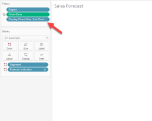
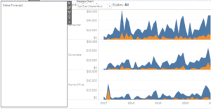
Step 5: On your Dashboard
– Select a ‘Vertical’ Pane from the left
– Add 1st sheet
– Add 2nd sheet and remove the ‘Title’
Notes:
– If you use a horizontal pane, you will need to remove the title from the 1st sheet
– If you use a vertical pane, you can keep the title on the 1st sheet and remove it from all
other sheets.
2nd sheet is blank and will seem to disappear. Once selected from your Parameter, it will populate
Step 6: Add the Parameter to your view as a Float dropdown list near the 1st sheet.
I hope this was helpful.